Statistical and mathematical strategies are applied in several areas for new product development.^1-3 In the chemical industry, these approaches are recommended and mainly used for evaluating the variables’ effects in a given system and for optimizing the manufacturing processes.^4-7 Several examples that employ statistical tools can be found in the literature: multivariate calibration, pattern recognition and design of experiments (DOE).^8-13 DOE has been used to organize the data set results from evaluation experiments and to obtain the maximum amount of information from a reduced number of experiments,^14,15 mainly when fractional factorial designs are performed.^16,17

Factorial design combines the use of mathematical and statistical knowledge to obtain information about a given system,¹⁸ and in chemistry this discipline is named chemometry.¹⁹ Lu et al.,²⁰ for instance, used full factorial design to study a film-coated photoreactor, and three variables were investigated. Dickens²¹ used DOE to study the performance of epoxy coating system using an accelerated test laboratory. In polymer system studies, Sáenz and Asua²² investigated five variables using two-level fractional factorial design to identify the region of experimental conditions in which monodispersed latexes could be prepared. Mishra et al.,²³ also using a fractional factorial design, verified the effects of six variables in the semi-continuous emulsion polymerization of methyl methacrylate. Lucchesi et al.²⁴ investigated 10 variables using fractional factorial design to study suspension polymerization of styrene, divinylbenzene, and N-(p-vinylbenzyl)-4,4-dimethylazlactone.

Doehlert design is a type of second order DOE,⁸ and its main advantage is the fact that variables can have a different number of levels, and the number of experiments is smaller than those observed in central composite design, for example. Therefore, researchers can customize the DOE to their needs, save time/reagents and get the same level of results as if they used central composite design.²⁵ Another well-established chemometric tool is principal component analysis (PCA), which is employed for exploratory analysis and compresses the raw data into a smaller number of variables named principal components (PC).^26‑28After PCA calculation, the data set is divided in two new matrices named scores and loadings. These matrices have information about samples (scores) and variables (loadings) and are analyzed together for better data interpretation and visualization.²⁷

Coatings have been used for different purposes, including covering substrates, adding value to products (automobiles, electronic equipment, buildings, e.g.) or protecting substrates (such as pipelines and bridges). One of the most important requirements for these applications is the quality of the final film. A continuous, crack-free, transparent and non-porous polymeric film can be considered to have the desired properties,^29-31 and these characteristics are proportional to the paint’s durability. Waterborne decorative coatings are complex formulations usually composed of latex, which can be defined as an aqueous colloidal dispersion of polymer micelles,³² water as solvent, pigments and additives, such as rheological modifiers and coalescents. When the environmental temperature is lower than the glass transition temperature (Tg) of the latex polymer, a defect or nonhomogeneous film formation is evident.^31-33 In this case, coalescents can be added to promote better film formation by allowing the fusion of latex micelles and by decreasing polymer Tg.^29,32,33 Coalescent selection is not an easy task and is typically based on experimental and empirical evaluations of film properties (scrub resistance, e.g.). Different variables on several levels often need to be studied.  Interactions among them are regularly neglected, and the formulator has no idea how many experiments need to be done.  In most cases, this question forces the coating formulator to prioritize one property against others according to their requirements.

The aim of this study is to demonstrate how powerful the combination of some statistical tools (Doehlert design and PCA) is to select the best latex to produce decorative coatings. In this case, empirical models were proposed and how they can be used was exemplified. The following film formation characteristics were evaluated: scrub resistance, minimum film formation temperature (MFFT) and drying time. Coalescent concentration, coalescent characteristics and latex type were the variables studied.

Experimental

Sample Preparation

In this study seven coalescent products (C) that are among the most well-known materials used in commercial waterborne decorative formulations, were selected for evaluation. The main differences among them were the chemical function, evaporation rate and water solubility. Coalescents were ordered from the least to the most water soluble and named: C1, C2, C3, C4, C5, C6 and C7. These coalescents were tested in concentrations ranging from 0 to 5.0% (w/w). All latexes used in this study were styrene acrylics and had different MFFTs and particle sizes. They were ordered from lowest to highest, based on Tg and identified as L1, L2, L3, L4 and L5. Therefore, variables for both coalescents and latexes were stipulated based on quantitative parameters, solubility in water and Tg, respectively. Actually, this strategy is not new, and some examples can be observed in the literature. McKie and Lepeniotis,³⁴ for instance, used a fractional factorial design in order to optimize the synthesis of poly(RS)-3,3,3-trifluorolactic acid, and one of the investigated variables was the catalyst. Other examples include Lima et al,³⁵ and Sadat-Shojai et al.³⁶

Samples were prepared by homogenizing coalescent with latex for 5 min in a Red Devil mixer. Sample analyses were performed after 24 h, and parameters were measured in triplicate for each experiment. All sample preparations and characterizations were carried out in Dow Brasil São Paulo R&D.

Scrub Resistance

Tests and procedures used in this study were the same as coating professionals apply to evaluate film formation, e.g., standard ASTM (American Society for Testing and Materials) and/or ABNT NBR (Brazilian Association of Technical Standards). As described in ASTM D 2486-0637 samples were applied using a 175 µmextensor on black scrub resistance panels (P 121-10N) and dried for 7 days at room temperature (~25 °C). The coated panel was then scrubbed with a bristle brush and an abrasive scrub with a BYK Gardner Abrasion Tester. The number of cycles necessary to remove the film in one continuous thin line across the shim was considered as “scrub resistance”. A high number of cycles means high scrub resistance and, consequently, homogeneous film formation (requested characteristic).

Minimum Film Formation Temperature (MFFT)

Samples were applied using a 175 µm extensor on plastic films under a temperature range (from 0 to 25 °C) in the MFFT equipment (Modern Metalcraft Co., USA). MFFT was determined by visual inspection of cracking and whitening in the film according to ASTM D 2354-98.³⁸ Low temperatures for MFFT mean that the coalescent will be more effective at promoting film formation, so a low MFFT is the expected condition for this test.

Drying Time

Samples were applied using a 175 µm extensor on glass plate. Drying time, recorded by a chronometer, was determined when the pendulum stopped stamping the film, according to standard ABNT NBR 15311:2005.39 Fast film formation was considered as the most favorable condition because of customer preferences towards faster coating application. DC 9610 Circular Gardner equipment was used, 360˚, 1 hour.

Experimental Design

Two Doehlert designs were prepared using the following variables: coalescent type (CT), coalescent concentration (CC) and latex type (LT). In the first design, the latexes, coalescent concentration and coalescent type were tested in 5, 7 and 3 levels, respectively. In the second, these same variables were investigated in 3, 5 and 7 levels, respectively. Both experimental sets were combined to obtain a global vision from the three variables’ effects. In this case, all variables were coded from -1 to +1, as presented in Table 1. A total of 36 experiments (experiments from 1 to 20 for Doehlert 1 and from 21 to 36 for Doehlert 2) were conducted, and some of them were performed in replicates (Table 1).

The statistical evaluations were performed using Microsoft Excel and/or JMP (version 8, from SAS Institute Inc.) software. Experimental results obtained for each test were normalized between 0 to 1 considering the desired results for each test as 1: high values for scrub resistance (SR) and small values for MFFT and drying time (DT). An average of normalized experimental results (A_results) for each experiment was calculated using the Equation 1 given weight 3 for both SR and MFFT and 1 for DT. These weights were given according to our manufacturer experience in the paint market. The customers are more interested in a film with a high scrub resistance property (high SR) that is able to be applied at any temperature (low MFFT).

An initial empirical model was proposed using the training data set (experiments from 1 to 13 and from 21 to 33, see Table 1), and 10 coefficients were calculated: b₀(intercept), b₁CT (linear coefficient for coalescent type), b₂CC, b₃LT, b₄CT² (quadratic coefficient for CT), b₅CC², b₆LT², b₇CTCC (interaction coefficient between CT and CC), b₈CTLT and b₉CCLT.

The modeled property (matrix Y) was the A_result (Equation 1 and Table 1). The previous-mentioned coefficients were calculated according to Equation 2.^14,15

X is a matrix containing the coded variables as presented in Table 1 (to calculate b₁to b₃), the quadratic terms (b₄to b₆) and the variables interactions (b₇to b₉). The constant (b₀) was a column with ones. Model accuracy was checked through ANOVA table. Sum of squares and mean squares, among other statistical parameters, were calculated based on applied statistical equations.^14,15,40

The model’s accuracy was verified by analyzing the root mean square error of prediction (RMSEP) for validation experiments. The validation experiments were not used in the training set and they are marked with an asterisk in Table 1: experiments from 14 to 20 and from 34 to 36. Equation 3 shows how the RMSEP values were calculated.

Where y_i and  ŷ_i, are the real and predicted values, and N_pred is the number of samples used in the validation set (10 samples in this case).

Results and Discussion

Empirical Model Using A_Results

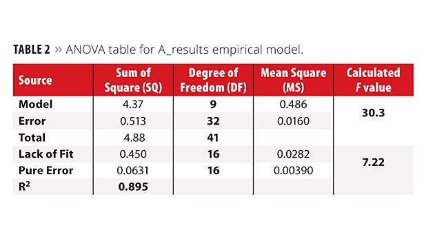
ANOVA table is presented for A_result empirical model on Table 2. As a total of 42 experiments were performed to compose the training data set, the degree of freedom (DF) for the total sum of square (SQ_Total) is 41 (42-1). In addition, 10 coefficients were calculated, and thus the DF for the model and error were 9 (10-1) and 32 (41-9), respectively. In order to compare these sources of variance, an F test was performed, taking into account the mean square for model (MS_Model) and the mean square for error (-MS_Error). This test is suitable to see the model quality, and the expected result is an F value higher than the tabulated one. For this particular case, the calculated F (30.3) was bigger than tabulated F_9,32 (2.19) with a 95%  confidence level.^14,15 This means that the model is valid, consistent and both MS are from different populations. In order to verify the prediction power of the model, mean square for lack of fit (MS_LOF) and mean square for pure error (MS_PE) were also evaluated. As 16 experiments from the training set were performed in authentic duplicate (Table 1), the DF for MS_PE is 16 and, in the case of MS_LOF, the DF is also 16 (32 (DF for MS_Error) – 16 (DF for MS_PE) = 16). When these mean squares are compared, a calculated F value lower than the tabulated one is expected, otherwise the model has problems with lack of fit. The calculated F (7.22) was bigger than tabulated F_16,16 (2.33) with a 95% confidence level, indicating that the proposed model is not well adjusted by the calculated coefficients and the MS_LOF (with DF = 16), instead of MS_Error (with DF = 32), must be used as variance to calculate the error for each coefficient. The correlation coefficient (SQ_Model/SQ_Total = R²) for this model was 0.895.

The calculated and valid coefficients (with 95% of confidence level) for the model using A_result are presented in Equation 4. In this case, only the intercept and the linear coefficients for coalescent concentration (CC) and latex type (LT) variables were valid.

The empirical model presented by Equation 4 is clearly poor because the information about the coalescent type (CT) was not taken into account. This observation was due to the fact that the model using A_result has lack of fit and it is not well adjusted to the real values. The coefficients presented in Equation 4 were used to calculate the predicted values, and the RMSEP was 0.315. This error is very high because the A_results were normalized up to 1.

PCA Approach

This initial model shows low prediction power, and a second approach was performed using principal component analysis (PCA) as a strategy for better understanding the data and to simplify the model.⁴¹ A matrix with all sample replicates (from 1 to 36), the coded variables (CC, CT and LT) and the A_results (Equation 1) was organized (156 rows and 4 columns). The data matrix was auto scaled to give the same importance to all variables and a PCA was performed. Using this pre-processing, the standard deviations for each variable are equal to 1, and the mean is 0. Figure 1 shows the scores plot for the first two principal components (PC1 and PC2), and coalescent concentration (Figure 1a), coalescent type (Figure 1b) and latex type (Figure 1c) categories are highlighted. These two PCs accounted for 78% of explained variance, and Figure 2 shows the loadings plot.

The first information that can be observed from the scores plots (Figures 1a-c) is the good reproducibility of the experiments performed because the three replicates for each experiment are clustered and in some cases overlapped.

Coalescent concentration category (see Figure 1a) values were displayed in three ranges: from 0 to 1% (triangles), from 1.7 to 2.5% (half tone circles) and from 3 to 5% (black squares). In Figure 1a, a separation is noted according to the coalescent concentrations. Samples with coalescent concentrations equal or lower than 1% (white triangles) are in the left bottom side of the plot. Samples with high coalescent concentration (equal or higher than 3, black squares) are in the right side of Figure 1a. The intermediate concentrations (from 1.7 to 2.5, half tone circles) are positioned between these two groups. When the coalescent type category is observed (Figure 1b) it is not possible to see a clear distinction among the coalescents used, except when the coalescent was not employed (N, stars). Figure 1c shows the latex type category highlighted, and a separation among latexes L1 and L2 (white triangles), L3 (half tone circles) and L4 and L5 (black squares) is observed in the PC2 axis. Latexes L1 and L2 had the lowest Tg values when compared with the other latexes.

Figure 2 shows the PC1 versus PC2 for loadings plot. The first PC has high contribution from both coalescent concentration (CC) and A_results variables. These two characteristics are related to high coalescent concentration (see Figure 1a). On the other hand, PC2 has high contribution from latex type (LT) and some from CC. With the help of these figures it is noted that the A_results have high positive values for PC1 loadings. In this case, those experiments with high and positive values for PC1 scores are associated with good experimental conditions (high SR and low MFFT and DT).

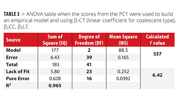
With this assumption, PC1 scores can be used to calculate an empirical model instead of A_results. The scores from the PC1 were then used as the Y matrix to calculate a model using the same coefficients previously mentioned in the Experimental Design section. Using this strategy the following three coefficients were significant: b₁CT (linear coefficient for coalescent type), b₂CC, b₃LT, at a confidence level of 95% and a new model using only these coefficients were calculated. Table 3 shows the ANOVA for this model. This model is superior to that mentioned previously because now the three variables studied present significant coefficients.

When the MS_Model and MS_Error were compared, the calculated F value (537) was bigger than the tabulated F_2,39 with a 95% confidence level (3.24).^14,15 The ratio between the calculated and tabulated F values was 166. This value is higher than that presented by the first model (14 using only A_results).  In addition, the R² was also improved and was 0.965 against 0.895 for the first model. For MS_LOF and MS_PE the calculated F (6.42) continues bigger than tabulated F_23,16 with 95% confidence (2.24).^14,15 It suggests the proposed model is not well adjusted to the calculated coefficients and the MS_LOF (with DF = 23) must be used as variance to calculate the error for each coefficient. Coefficients were calculated for the model and only the valid ones with 95% confidence are presented in Equation 5.

Equation 5 shows that only the linear coefficients (CC, CT and LT) were valid. Now, as expected, the CT variable is important for the model. Based on this equation, PC1 scores values and its standard deviation were calculated for validation experiments (14 to 20 and 34 to 36). The predicted values were converted into predicted A_results based on direct correlation among scores from PC1 and experimental A_results calculated only using samples from the calibration set (Equation 6).

Predicted values from PC model were compared with real A_results, and the RMSEP was 0.234 (lower than that showed in the first model).

Application of the Proposed Model Combining Doehlert Design and PCA

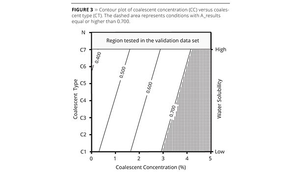
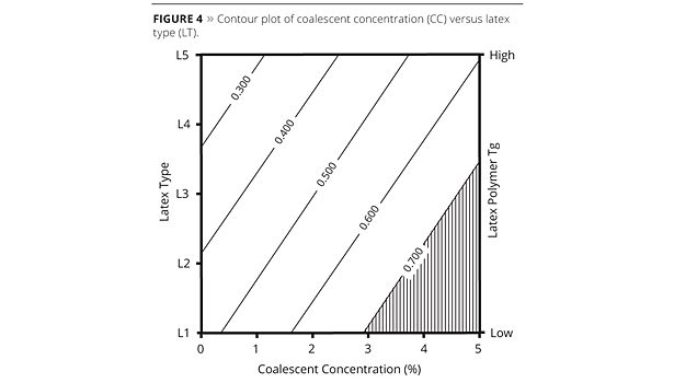
In order to visualize the model, contour plots were prepared based on direct correlation between the A_results and PC1 scores (Figures 3, 4 and 5). The desirable A_results (high values) were highlighted for each plot. In this case the area with values higher than 0.700 was selected.

For CC versus CT contour plot (Figure 3) the coalescent water solubility axis was added at the right side of the plot for better visualization. Desirable conditions (high results) in this case means that any coalescent can be used (from C1 to C7) at concentrations higher than 4%. Coalescents with the lowest water solubility, such as C1, C2 and C3, may be used in concentrations lower than 4% and higher than 3% to generate the same film quality. Coalescent concentration against LT contour plot (Figure 4) shows correlation among latex type and polymer Tg increasing at the right axis. Desirable conditions were obtained using the following latex:  L1, L2 or L3. These latexes have the lowest Tg and can be used with coalescent concentrations equal to, or higher than, 3% (for L1), 4% (for L2) and 5% (for L3). The latex L1, for example, presented better results even when a lower coalescent concentration (2.5%) was used, as can be observed in experiment 5 (see Table 1). The contour plot of LT versus CT (Figure 5) has, respectively, coalescent water solubility and latex polymer Tg order indication on the axis. Latex L1 or L2 and coalescent C1 combination generated the desirable work condition. This model can be improved taking into account other factors, such as cost, for example. In addition, the model can be updated when new materials (coalescents and latexes) are available in the market.

Conclusions

The impact of coalescent type, coalescent concentration and latex type variables on film formation were investigated through the application of key statistical tools. Two Doehlert designs were carried out using scrub resistance, MFFT and drying time as evaluated conditions. Experimental results from each test were normalized, between 0 and 1, and a weight average was calculated according to the decorative coating market preferences. The final result was a model where the researcher can identify the best material for a given emulsion. The model can be improved with the use of other parameters like cost of production and product characteristics.

Author's note: This study was conducted during the project of Professional Master course of Marcelo B. Graziani.

Acknowledgements

The authors are grateful to the Conselho Nacional de Desenvolvimento Científico e Tecnológico (CNPq).

References

¹     Pichavant L.,; Coqueret X. Optimization of a UV- curable acrylate-based protective coating by experimental design. Prog Org Coat, 63, 55-62 (2008).

²     Emélie B.; Schuster U.; Eckersley S. Interaction between styrene/butalacrylate latex and water-soluble associative thickener for coalescent free wall paints. Prog Org Coat, 34, 49-56 (1984).

³     Pereira FMV, Bueno MIMS. Image evaluation with chemometric strategies for quality control of paints. Anal Chim Acta, 588, 184-191 (2007).

⁴     Pereira FMV, Bueno MIMS. Calibration of paint and varnish properties: potentialities using X-ray spectroscopy and partial least squares. Chemom Intell Lab Syst, 92, 131-137 (2008).

⁵     Farzaneh A.; Ehteshamzadeh M.; Ghorbani M.; Mehrabani J.V. Investigation and optimization of SDS and key parameters effect on the nickel electroless coatings properties by Taguchi method. J Coat TechnolRes, 7, 547-555 (2010).

⁶     Sabadini E.; Hubinger, M.D.; Cunha, R.L. The effects of sucrose on the mechanical properties of acid milk. J. Chem. Eng., 23, 55-65 (2006).

⁷     Pleterski, M.; Tusek, J.; Muhic, T.; Kosec, L. Laser cladding of cold-work tool steel by pulse shaping. J. Mater. Sci. Technol., 27, 707-713 (2011).

⁸     Ferreira, SLC.; Santos, WNL.; Quintella, C.M.; Barros, Neto B.; Bosque-Sendra, J.M. Doehlert matrix: a chemometric tool for analytical chemistry – review. Talanta, 63, 1061-1067, (2004).

⁹     Ferreira, SLC.; Bruns, R.E.; Ferreira, H.S.; Matos, G.D.; David, J.M.; Brandão, G.C.;Silva, EGP.; Portugal, L.A.; Reis, P.S.; Souza, A.S.; Santos, WNL. Box-Behnken design: An alternative for the optimization of analytical methods. Anal Chim Acta, 597,179-186, (2007).

¹⁰    Muteki, K.; MacGregor, J.F.; Ueda, T. Mixture designs and models for the simultaneous selection of ingredients and their ratios. Chemom Intell Lab Syst,86, 17-25 (2007).

¹¹    Prendi, L.; Ali, A.; Henshaw, P.; Mancina, T.; Tighe, C. Implementing DOE to study the effect of paint application parameters, film build, and dehydration temperature on solvent pop. J Coat TechnolRes, 5, 45-56 (2008).

¹²    Wery, S.; De Petris-Wery, M.; Feki, M.; Ayedi, HF. Application of a factorial design to study a chromate-conversion process. J Coat Technol Res, 7, 39-47 (2010).

¹³    Oktem, H.; Erzurumlu, T.; Uzman, I. Application of Taguchi optimization technique in determining plastic injection molding process parameters for a thin-shell part. Mater Des, 28, 1271-1278 (2007).

¹⁴    Bruns, R.E.; Scarminio, I.S.; Barros Neto, B. Statistical Design – Chemometrics: Data Handling in Science and Technology. Elsevier, Amsterdam (2006).

¹⁵    Montgomery, D.C. Design and Analysis of Experiments. John Wiley & Sons: Hoboken (2005).

¹⁶    Solvason, C.C.; Chemmangattuvalappil, N.G.; Eljack, F.T.; Eden, M.R. Efficient Visual Mixture Design of Experiments Using Property Clustering Techniques. Ind Eng Chem Res, 48, 2245-2256 (2009).

¹⁷    Santos, J.S.; Trivinho-Strixino, F.; Pereira, E.C. Investigation of Co(OH)2 formation during cobalt electrodeposition using a chemometric procedure. Surf Coat Technol, 205, 2585-2589 (2010).

¹⁸    Nahui, F.N.B.; Nascimento, M.R.; Cavalcanti, E.B.; Vilar, E.O.; Braz J. Chem. Eng., 25, 435-442 (2008).

¹⁹    Leardi, R. Experimental design in chemistry: A tutorial. Anal Chim Acta, 652, 161-172 (2009).

²⁰    Lu, P.J.; Chien, C.W.; Chen, T.S.; Chern, J.M. Azo dye degradation kinetics in TiO2 film-coated photoreactor. Chem Eng J, 163, 28-34 (2010).

²¹    Dickens, B. Model-free estimation of outdoor performance of a model epoxy coating system using accelerated test laboratory data. J Coat TechnolRes, 6, 419-428 (2009).

²²    Sáenz, J.M.; Asua, J.M. Dispersion copolymerization of styrene and butyl acrylate in polar solvents. J Polym Sci Part A: Polym Chem34, 1977-1992 (1996).

²³    Mishra, S.; Singh, J.; Choudhary, V. Factorial Experimental Design Approach in Semicontinuous Emulsion Polymerization of Methyl Methacrylate to Study the Effect of Process Variables. J Polym Sci Part A: Polym Chem, 113, 3742-3749 (2009).

²⁴    Lucchesi, C.; Pascual, S.; Jouanneaux, A.; Dujardin, G.; Fontaine, L. Tuning the Parameters of the Suspension Polymerization of Styrene, Divinylbenzene, and N-(p-vinylbenzyl)-4,4-dimethylazlactone. J Polym Sci Part A: Polym Chem, 45, 1977-1992 (2007).

²⁵    Bezerra, M.A;.. Santelli, R.E.; Oliveira E.P., Villar, L.S.; Escaleira, L.A. Response surface methodology (RSM) as a tool for optimization in analytical chemistry, Talanta, 76, 965 (2008).

²⁶    Wold, S.; Esbensen, K.; Geladi, P. Principal component analysis. Chemom Intell Lab Syst,2, 37-52 (1987).

²⁷    Sharaf, M.A.; Illman, D.L.; Kowalski, B.R. Chemometrics. John Wiley & Sons: New York, (1986).

²⁸    Massart, D.L.; Vandeginste, BGM; Buydens, LMC; De Jong, S.; Lewi, P.J.; Smeyers-Verbeke J. Handbook of Chemometrics and Qualimetrics: Part A. Elsevier: Amsterdam (1997).

²⁹    Vanderhoff, J.W.; Bradford, E.B.; Carrington, W.K. The transport of water through latex films. J Polym SciPolym Symp, 41, 155-174 (1973).

³⁰    Toussaint, A.; De Wilde, M.; Molenaar, F.; Mulvihill, J. Calculation of Tg and MFFT depression due to added coalescing agent. Prog Org Coat, 30, 179-184 (1997).

³¹    Toussaint, A.; De Wilde, M. A comprehensive model of sintering and coalescence of unpigmented latex. Prog Org Coat, 30, 113-126 (1997).

³²    Keddie, J.L. Reports: A Journal Review Film Formation of Latex. Mater Sci Eng Rep,21, 101-170 (1997).

³³    Kiil, S. Drying of Latex films and Coatings: Reconsidering the Fundamental Mechanisms. Prog Org Coat, 57, 236-250 (2006).

³⁴    McKie, D.B.; Lepeniotis, S. Optimization techniques for carbodiimide activated synthesis of poly ((RS) – 3,3,3-trifluorolactic acid; statistically designed experiments to optimize polymerization conditions. Chemom Intell Lab Syst, 41, 105-113 (1998).

³⁵    Lima, L.F.; Corraza, M.L.; Cardozo-Filho, L.; Márquez-Alvarez, H.; Antunes, OAC. Oxidation of limonene catalyzed by metal(salen) complexes. Braz J. Chem. Eng., 23, 83-92 (2006).

³⁶    Sadat-Shojai, M.; Atai, M.; Nodehi, A. Design of experiments (DOE) for the optimization of hydrothermal synthesis of hydroxyapatite nanoparticles. J Braz Chem Soc22, 571-582 (2011).

³⁷    ASTM standard “Standard Test Methods for Scrub Resistance of Wall Paints”, D 2486-06, Annual Book of ASTM Standards (2006).

³⁸    ASTM standard “Standard test method for Minimum Film Formation Temperature (MFFT) of emulsion vehicles”, D 2354-98, Annual Book of ASTM Standards (1998).

³⁹    ABNT standard. “Paints for buildings - Method for performance evaluation of paints for non industrial buildings - Determination of drying time of paints and varnishes by instrumental method”, NBR 15311:2005, (2005).

⁴⁰    Box, G.E.P.; Hunter, W.G.; Hunter, J.S. Statistics for experimenters An introduction to design, data analysis, and model building. John Wiley & Sons, New York (1978).

⁴¹             Bezerra, M.A.; Bruns, R. E.; Ferreira, S.L.C. Statistical design-principal component analysis optimization of a multiple response procedure using cloud point extraction and simultaneous determination of metals by ICP OES, Anal Chim Acta, 580, 251-257 (2006).