Using Design of Experiments to Make Processes More Robust to Environmental and Input Variations
Parameter Design Advocated by Taguchi (Two-Array)
In the early 1980s, the methods of Genichi Taguchi became popular as a tool for quality improvement, especially in the automotive industry. Taguchi provided a focus on robust design that reached fruition in the Six Sigma movement. The basic philosophy of robust design is that it is desirable to develop processes that consistently produce product to target with minimal variation.To achieve this objective, Taguchi advised that input variables be divided into two categories: control factors, such as the adjustments a technician makes to your office copier, and noise factors, such as the humidity that fluctuates in your office environment.
Ideally, processes will be adjusted by way of the control factors to be insensitive to the noise factors, whose variation presumably cannot be eliminated. For example, the office copy machine should handle paper properly during humid summer months as well as in the winter, when conditions are dry and prone to static electricity. To accomplish these objectives, Taguchi advocated planned experimentation using a layout called "parameter design."1
In this case, the objective is to consistently apply a coating by way of three control factors: sanding, thickness of application, and depth of primer layer.
- Time
Temperature
Relative humidity
Ultraviolet (UV) exposure.
In general, a parameter design is composed of two parts: An inner array of control factors and an outer array of noise variables.
Table 1 shows the parameter design that we propose for the connector case. As noted below, it varies somewhat from that shown by Taguchi and his disciples (such as Ross).
- 1. The control factors are studied by way of a full two-level factorial design (23), which provides complete resolution of all effects. The eight runs are listed in standard ("Std.") order, which differs from that used by Taguchi.
2. The noise variables go into a standard half-fraction two-level design (24-1). This design resolves main effects fairly well, but it leaves two-factor interactions aliased.2 The eight runs in this portion of the parameter design (the outer array) are also listed in standard order.
The levels in both arrays are coded minus (-) and plus (+) for the low and high levels, respectively, rather than the numbers 1 and 2 used by Taguchi for what he calls the first and second levels. The number of runs in the parameter design for the connector case totals 64 (8 inner x 8 outer).
Whenever practical, the actual runs in any DOE should be done in random order, which avoids possible confounding of effects with time-related lurking variables, such as machine wear. In any case, after collecting all the raw data, the experimenter should then calculate the mean and standard deviation ("Std. Dev."). We recommend that these summary statistics be analyzed separately before putting them in the form of a ratio, such as Taguchi's signal-to-noise, thus preserving valuable information that might otherwise be lost. The significant factors, identified by way of analysis of variance (ANOVA), will fall into one of four classes1 affecting the following.
- I. Both average (mean) and variation (standard deviation)
II. Variation only
III. Average only
IV. Nothing.
Parameter design accomplishes the goal of determining a setup of control factors that will be robust to variations caused by noise factors. However, this experiment can be designed in such a way that reveals essentially as much information on the effects of control factors and noise variables, but with only half the data.
Alternative Design that Combines All Factors into One Array
Let's look at an alternative design option for the coating study. It combines all the factors, control and noise, into one two-level factorial array (see Table 2). This design, a standard quarter-fraction (27-2), requires only 32 runs.The complete alias structure for this design can be seen in textbooks2 so we won't show it all here. All main effects can be estimated clearly because they're aliased only with interactions of three or more factors, which by common practice are assumed to be negligible. Furthermore, all two-factor interactions involving A, B or C (the control factors) are also aliased only with three-factor interactions, so they can be relied upon as well. The only aliasing of any concern occurs among the noise variables - D, E, F and G.
- [DE] = DE + FG
[DF] = DF + EG
[DG] = DG + EF
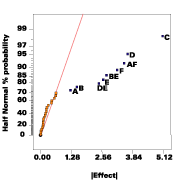
The labeled effects are statistically significant with more than 99.99% confidence according to analysis of variance (ANOVA). (We did a good job on the simulation!) Before interpreting the results, it will help to categorize factors as follows.
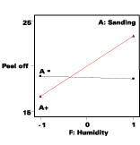
- 1. Control factors involved in interactions with noise variables (A with F, B with E)
2. Control factors not involved in interactions with noise variables (C)
3. Noise variables not involved in interactions with control factors (D)
4. Control factors that have no effect (none in this case)
5. Noise variables that have no effect (G)

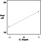
Setting A and B to minimize variation make these two factors inflexible for controlling the response. That's where factor C (depth) comes into play. It falls into the second category of factors that do not interact with noise variables. The effect of C is shown in Figure 3.

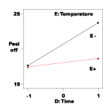
Finally, look at noise variables that do not interact with control factors. In this case, variable D (time) falls in this category as well as the interaction effect (DE). Remember that DE is aliased with FG in this design, so we can't be sure that DE really does create an effect. However, one of the parent terms of FG, G (UV exposure), does not exhibit significant effects. On the other hand, both D and E are significant, so it's a good bet that their 'child,' DE, really is the significant interaction rather than its alias - FG.
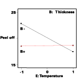
What, if anything, can be done when a process is significantly affected by noise variables? The obvious answer is to impose control. For example, in this case nothing can be done about the time (D) the part is kept in storage, but temperature (E) in the warehouse could be controlled with the proper equipment. The high level (E+) moves the response to the flat line on the interaction graph (see Figure 4), which will be robust to the affects of varying time, so it would be wise to invest in some space-heating (it gets cold in Minnesota!). This will put the process that much closer to conformance with Six-Sigma objectives.

As a postscript to the story, note that there may be control factors that are not significant (category 4). You may be tempted to set these factors at levels that are most economical or convenient for operation, but that would not be consistent with the objectives of robust design. It's best to leave the insignificant factors at their mid-level in case they might vary. Ideally, such variation will occur within the experimental range and thus should not affect the process.
Similarly, some noise variables, such as the exposure to UV, may not create significant effects on the response (category 5). At the very least, this might justify leaving these variables uncontrolled. For example, in this case, it appears that there would be no advantage to spending money on new, UV-resistant packaging for the coated parts.
Response Surface Methods (RSM) and Measurement of Propagation of Error (POE)
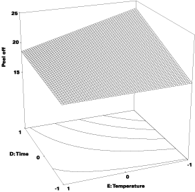
A more advanced approach to robust design makes use of response surface methods.4 Figure 5 shows an example of a response surface generated from the interaction DE in the coatings case.Consider how variations in time get transmitted to the response (peel-off). These variations will be substantially reduced at the flatter portion of the surface (in front), where temperature gets set at its high (+1) level. A mathematical tool called propagation of error (POE) can be applied to quantify the error transmitted by way of the response surface from the variations in input factors, which must be determined beforehand from repeatability studies, SPC or ANOVA on prior DOE data.5
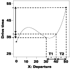
To get a feel for POE, consider a very simple, fun and practical example: driving through rush-hour traffic.6 Figure 6 shows how timing is everything if you want to get to work consistently on time. It shows how drive time (in minutes) varies as a function of the time of departure (minutes after 6:30 A.M.). Notice the waviness that occurs due to traffic patterns. Assume that the driver won't leave exactly at the targeted departure time - this will vary over a 10-minute window. That variation in departure will be transmitted by way of the response curve to the drive time. At T1 this variation is very slight (see the small arrow on the drive time axis). However, only a short while later at T2, the variation gets amplified (see the big arrow on drive time) by the steep curve that results from daily traffic jams in the heart of the rush hour.
RSM generates polynomial models to fit data such as that collected on drive time. The model used to create the curve in Figure 6 is cubic:
Drive time = Y = 32.13 + 1.72X - 0.102X2 + 0.00159X3
When the model reveals curvilinear relationships between controllable factors and responses, such as the drive time case, transmitted variation can be reduced by moving to plateaus. The catch phrase for robust design, as stated earlier, is "find the flats." These can be located by generating the POE, which involves some calculus.5 The first step is calculation of the response variance (dy2):
dy2 = (dY/dX)2 dX2 + de2
where dX2 is the variance of the input factor X and de2 is the residual variance that comes from the analysis of variance (ANOVA). In the drive time case these values are:
- dX2 = (5 minutes)2 = 25
de2 = Mean square residual from ANOVA = 5.18
dY/dX = 1.72 - 0.204X + 0.00477X2
The POE is conveniently expressed in the original units of measure (minutes of drive time in this case) by taking the square root of the variance of response Y by way of this final equation:
POE = [dy2]0.5 = [(dY/dX)2 dX2 + de2]0.5 = [(1.72 - 0.204X + 0.00477 X2)2*25+5.18]0.5
With the aid of software3, the POE can be calculated, mapped and visualized. Figure 7 shows the POE for the drive time case study. It exhibits two local minima, one for the peak at 11.5 (a high 'flat' point in Figure 6) and one for the valley at 31.5 (a low 'flat' point).
The drive time example involves only one factor. Generally, robust design by way of RSM involves more than one factor. In fact, for purposes of robust design, the experimenter should try to include control factors and noise variables thought to be significant based on past experience (prior DOE) or subject matter knowledge. Ideally, the analysis will reveal that factors affect the response in various ways: Non-linear (curved surface) or linear.
The non-linear factors, such as storage temperature in the coatings case, should be set at levels that minimize POE. On the other hand, Figure 8 shows the variation transmitted by a linear factor (X2) will be constant, so POE becomes irrelevant.
Therefore, linear factors can be freely adjusted to bring the response into specification while maintaining the gains made in reducing variation by way of POE on the non-linear factors. The ideal case is represented by Figure 9. The top curve represents production before applying the tools of robust design. With information gained from POE analysis, the experimenter can adjust the non-linear factor(s) to minimize process variation. This tightens the distribution as shown by the middle curve in Figure 9. However, average response now falls off target. Therefore, a linear factor, such as X2 in Figure 8, must be adjusted to bring the process back into specification (the "After" curve). Thus, the mission of robust design and Six Sigma is accomplished.
Conclusion
As shown by example, standard two-level fractional factorials (one array, 2k-p) are more efficient and provide more information than the two-array parameter designs advocated by Taguchi. For any given parameter design, it will be worthwhile to investigate alternative 2k-p designs to see if the number of runs can be reduced and/or more effects resolved, particularly those involving interactions of noise variables. If control can be imposed on certain noise variables, the effects of other noise variables might be reduced. This information would likely be lost in the overly simplistic approach of parameter design, which somewhat arbitrarily distinguishes control factors from noise variables.
Experimenters should consider how much variation can be anticipated in all the variables. This data, typically entered in the form of standard deviations, can then be made use of in the calculation of propagation of error (POE). POE, in conjunction with response surface methods (RSM), facilitates the search for robust operating regions - the flats where variations in input factors do not get transmitted much to the response. The end-result of applying these advanced tools will be in-specification products that exhibit minimal variability - the ultimate objective of robust design and Six Sigma.
Acknowledgements
The authors thank their colleague Patrick Whitcomb for many valuable suggestions and much of the source material for this paper.For more information on design of experiments, contact Mark@StatEase.com or Shari@StatEase.com; or visit www.StatEase.com.
References
1 Ross, P.J. 1988. Taguchi Techniques for Quality Engineering. New York: McGraw-Hill.2 Anderson, M.J.; Whitcomb. P.J. 2000. DOE Simplified, Practical Tools for Experimentation. Portland, Oregon: Productivity Inc.
3 Helseth, et. al. 2002. Design-Expert(r) Software, Version 6, Minneapolis: Stat-Ease Inc.
4 Myers, R.H.; Montgomery, D.C. 2002. Response Surface Methodology, 2nd Edition, New York: John Wiley.
5 Anderson, M.J.; Whitcomb. P.J. 1996. Robust Design - Reducing Transmitted Variation. Proceedings from the 50th Annual Quality Congress. Pages 642-651. Milwaukee: American Society of Quality.
6 Anderson, M.J., 2002. Six Sigma for Steel-Belts. Stat-Teaser newsletter, March 2002. Minneapolis: Stat-Ease Inc.
Links
Looking for a reprint of this article?
From high-res PDFs to custom plaques, order your copy today!
